
Tomographic Particle Imaging Velocimetry (Tomo-PIV)


The Tomographic Particle Image Velocimetry method is a relatively new extension of the PIV measurement technique with the specific ability to determine three-dimensional velocity vector fields [1]. Analogous to the planar PIV technique the principle of Tomo-PIV is based on the calculation of the velocity vector field in a flow from the displacement of imaged tracer particles (s.c. seeding) on two subsequently captured images of the region of interest. With a planar stereoscopic PIV set-up it is possible to determine instantaneous velocity vector fields with all three components in a two dimensional plane (2D-3C). Furthermorer, Tomo-PIV enables the determination of an instantaneous velocity vector volume (3D-3C).
The method is making use of the tomographic reconstruction of an instantaneous particle distribution based on the projections of this distribution onto several cameras: tiny tracer particles are added to the flow of interest and illuminated with a short laser light pulse in a volume with a rectangular base area. The light scattered by the particles is captured by several (ca. 3 to 6, typically 4) cameras applying the Scheimpflug condition. In that way weighted projections of the instantaneous particle distribution are received by the camera sensors from different viewing directions (see Fig. 1 [3]). The information about the lines of sight of each camera pixel through the investigated volume is described by a polynomial approximation achieved from a 3D-calibration procedure.
In a second step the original three-dimensional particle distribution has to be (re-)calculated from the projections to the cameras. Therefore the MART (Multiplicative Algebraic Reconstruction Technique) method is used, introduced by Herman und Lent [2]. The problem of reconstruction is converted into an under-determined system of equations, which can be solved in a converged approximation using algebraic methods. At the end of the reconstruction process a digital representation of the volume in the shape of a voxel space (deduced from pixel = picture elements -> volume elements) is obtained, in which intensity values virtually describe the original particle distribution.
The illumination and imaging of the volume within the flow is carried out at two subsequent time steps and a tomographic reconstruction for both time steps is performed. By calculating the three-dimensional cross-correlation of the obtained voxel-spaces locally on a regular grid a displacement vector field of the reconstructed particle distributions can be achieved analogous to the 2D-PIV evaluation process. A sketch summarizing the Tomo-PIV method is shown in Fig. 2 (after F. Scarano, TU Delft).
Applications
Tomo-PIV can be applied in air as well as in water. Like for planar PIV time-resolved experiments can be performed using high speed-cameras and –lasers. The fluid structure distributions are visualized e.g. by selected vector planes and 3D-iso-contour surfaces of the vorticity.
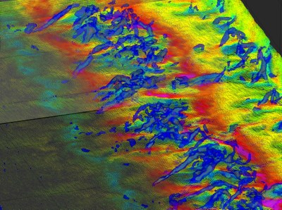
In case a time-resolved measurement is not necessary or higher spatial resolution is desired the application of high resolution double-frame cameras enables a measurement of instantaneous velocity distributions containing several scales within a complex flow simultaneously. Fig. 3 shows a result from an experiment in which four 16-Megapixel-cameras have been used for the imaging of a volume of 100 x 70 x 8 mm³ size in a transitional shear flow behind a Backward-Facing-Step. Vector fields with a spatial resolution of 1.1 independent vectors per mm³ have been achieved (resulting in a total number of more than 3.5 mio vectors per measurement point at 75 % overlap).
Future applications of Tomo-PIV in industrial wind tunnels will most likely be restricted to so called Fat-Sheet Tomo-PIV due to the influences of long viewing distances and vibrations of the cameras. With such a set-up it is possible to correct for the line-of-sight variations between the cameras by volume self-calibration [4] from single simultaneous images of each camera. The light sheet thickness is only slightly increased compared to a Stereo-PIV set-up, but results of a Fat-sheet Tomo-PIV measurement can deliver the complete instantaneous velocity gradient tensor in a “thick plane”.
Literature
[1] Elsinga G.E., Scarano F., Wieneke B. and van Oudheusden B.W. (2006); Tomographic particle image velocimetry. Exp Fluids 41:933-947(15)
[2] Herman G.T., Lent A.; Iterative reconstruction algorithms. Comput Biol Med 6:273–294, 1976
[3] Schröder A., Geisler R., Elsinga G.E., Scarano F., Dierksheide U. (2008); Investigation of a turbulent spot and a tripped turbulent boundary layer flow using time-resolved tomographic PIV. Exp Fluids 44:305–316
[4] Wieneke B. (2008); Volume self-calibration for 3D particle image velocimetry. 549-556, Exp Fluids 45:549–556